Figure 2b#
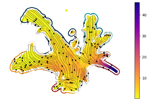
Velocity stream plot: LARRY dataset#
Here we’ll use the function sdq.pl.velocity_stream to plot the drift vector field and overlay this with the magnitude of diffusion. These plots give us an intuitive sense for the relative (low-dimension) direction of cell change alongside the magnitude of stochastic change. We’ll apply this plot to the LARRY dataset, performing the necessary prerequisite operations, including the following functions:
sdq.tl.drift(accessed also asmodel.drift()wheremodelis ansdq.scDiffEqmodel.sdq.tl.diffusion(accessed also asmodel.diffusion()wheremodelis ansdq.scDiffEqmodel.sdq.tl.velocity_graph
Import libraries#
[1]:
%load_ext nb_black

import scdiffeq as sdq
import pathlib
import cellplots as cp
import matplotlib.pyplot as plt
import larry

larry_cmap = larry.pl.InVitroColorMap()._dict

print(sdq.__version__, sdq.__path__)
0.1.1rc0 ['/home/mvinyard/github/scDiffEq/scdiffeq']
Load data#
[2]:
h5ad_path = (
    "/home/mvinyard/data/adata.reprocessed_19OCT2023.more_feature_inclusive.h5ad"
)
adata = sdq.io.read_h5ad(h5ad_path)
AnnData object with n_obs × n_vars = 130887 × 2492
    obs: 'Library', 'Cell barcode', 'Time point', 'Starting population', 'Cell type annotation', 'Well', 'SPRING-x', 'SPRING-y', 'clone_idx', 'fate_observed', 't0_fated', 'train'
    var: 'gene_ids', 'hv_gene', 'must_include', 'exclude', 'use_genes'
    uns: 'fate_counts', 'h5ad_path', 'time_occupance'
    obsm: 'X_clone', 'X_pca', 'X_umap', 'cell_fate_df'
    layers: 'X_scaled'
Load the model checkpoint#
Here, we’ll use a model checkpoint that was trained on the full LARRY dataset (further studied in Figure 4).
[3]:
ckpt_path = pathlib.Path(
    "/home/mvinyard/experiments/LARRY.full_dataset/LightningSDE-FixedPotential-RegularizedVelocityRatio/version_0/checkpoints/last.ckpt"
)
model = sdq.io.load_model(adata=adata, ckpt_path=ckpt_path)
 - [INFO] | Input data configured.
 - [INFO] | Bulding Annoy kNN Graph on adata.obsm['train']
Seed set to 0
- [INFO] | Using the specified parameters, LightningSDE-FixedPotential-RegularizedVelocityRatio has been called.
Compute the snapshot drift and diffusion#
We’ll call the operations using the functions built into the model class. This will pass the data stored in the model.adata object through the functions. These can also be called independently on a different adata object through the sdq.tl. part of the API.
[4]:
model.drift()
model.diffusion()
 - [INFO] | Added: adata.obsm['X_drift']
 - [INFO] | Added: adata.obsm['drift']
 - [INFO] | Added: adata.obsm['X_diffusion']
 - [INFO] | Added: adata.obsm['diffusion']
Smooth the data using kNN
[5]:
smoother = sdq.tl.kNNSmoothing(model.adata)
model.adata.obs["smooth.diffusion"] = smoother("diffusion")
df_inspect = model.adata.obs[["diffusion", "smooth.diffusion"]]
df_inspect.min(), df_inspect.max()
[5]:
(diffusion           0.202671
 smooth.diffusion    0.264766
 dtype: float32,
 diffusion           99.265465
 smooth.diffusion    45.804302
 dtype: float32)
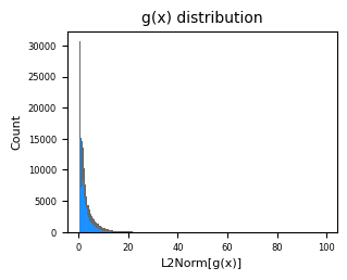
[6]:
fig, axes = cp.plot(
    height=0.5,
    width=0.5,
    title=["g(x) distribution"],
    x_label=["L2Norm[g(x)]"],
    y_label=["Count"],
)
b2 = axes[0].hist(model.adata.obs["diffusion"], bins=210, color="dimgrey")
b1 = axes[0].hist(model.adata.obs["smooth.diffusion"], bins=210, color="dodgerblue")
Compute velocity graph and plot#
We’ll use the velocity components we’ve just computed to compute the velocity graph that will ultimately enable us to build a low-dimension vector field.
Note: Since we’ve performed these operations on the model.adata object, we’ll use that in this function, directly.
[7]:
sdq.tl.velocity_graph(model.adata)
 - [INFO] | Added: adata.obsp['distances']
 - [INFO] | Added: adata.obsp['connectivities']
 - [INFO] | Added: adata.uns['neighbors']
 - [INFO] | Added: adata.obsp['velocity_graph']
 - [INFO] | Added: adata.obsp['velocity_graph_neg']
The following is the plot shown in Figure 2b of the manuscript.
[8]:
fig, axes = cp.plot(1, 1, height=1, width=1.2, del_xy_ticks=[True], delete="all")
ax = axes[0]
axes = cp.umap_manifold(
    adata,
    groupby="Cell type annotation",
    c_background=larry_cmap,
    ax=ax,
    s_background=350,
    s_cover=200,
)
sdq.pl.velocity_stream(
    model.adata,
    c="smooth.diffusion",
    cutoff_percentile=0.1,
    ax=ax,
    scatter_zorder=101,
    stream_zorder=201,
    scatter_kwargs={"rasterized": True},
)
plt.savefig("LARRY.example_velocity_stream.svg", dpi=500)