Figure S4#
Decomposing drift-diffusion-based velocity#
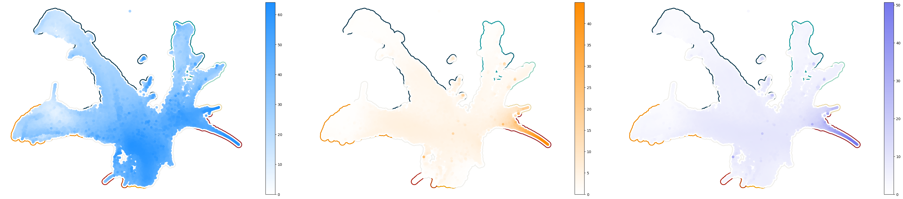
Here we examine the decomposed drift and diffusion of scDiffEq fit to the LARRY dataset.
Import libraries#
[1]:
%load_ext nb_black

import numpy as np
import pandas as pd
import matplotlib.cm as cm
import scdiffeq as sdq
import pathlib
import cellplots as cp
import matplotlib.pyplot as plt
import larry
import scdiffeq_analyses as sdq_an

larry_cmap = larry.pl.InVitroColorMap()._dict

print(sdq.__version__, sdq.__path__)
0.1.1rc0 ['/home/mvinyard/github/scDiffEq/scdiffeq']
Load data#
[2]:
h5ad_path = (
    "/home/mvinyard/data/adata.reprocessed_19OCT2023.more_feature_inclusive.h5ad"
)
adata = sdq.io.read_h5ad(h5ad_path)
AnnData object with n_obs × n_vars = 130887 × 2492
    obs: 'Library', 'Cell barcode', 'Time point', 'Starting population', 'Cell type annotation', 'Well', 'SPRING-x', 'SPRING-y', 'clone_idx', 'fate_observed', 't0_fated', 'train'
    var: 'gene_ids', 'hv_gene', 'must_include', 'exclude', 'use_genes'
    uns: 'fate_counts', 'h5ad_path', 'time_occupance'
    obsm: 'X_clone', 'X_pca', 'X_umap', 'cell_fate_df'
    layers: 'X_scaled'
Load the model checkpoint#
Here, we’ll use a model checkpoint that was trained on the full LARRY dataset (further studied in Figure 4).
[14]:
project_path = pathlib.Path(
    "/home/mvinyard/experiments/LARRY.full_dataset/LightningSDE-FixedPotential-RegularizedVelocityRatio"
)
project = sdq.io.Project(project_path)
[145]:
results = sdq_an.parsers.summarize_best_checkpoints(project)
results
[145]:
| train | test | ckpt_path | epoch | |
|---|---|---|---|---|
| version_0 | 0.552548 | 0.508731 | /home/mvinyard/experiments/LARRY.full_dataset/... | 970 |
| version_1 | 0.573248 | 0.54482 | /home/mvinyard/experiments/LARRY.full_dataset/... | 1499 |
| version_2 | 0.579618 | 0.51688 | /home/mvinyard/experiments/LARRY.full_dataset/... | 2457 |
| version_3 | 0.584395 | 0.542491 | /home/mvinyard/experiments/LARRY.full_dataset/... | 2500 |
| version_4 | 0.574841 | 0.549476 | /home/mvinyard/experiments/LARRY.full_dataset/... | 2153 |
[18]:
ckpt_path = results.loc["version_2"]["ckpt_path"]
model = sdq.io.load_model(adata=adata, ckpt_path=ckpt_path)
 - [INFO] | Input data configured.
 - [INFO] | Bulding Annoy kNN Graph on adata.obsm['train']
Seed set to 0
- [INFO] | Using the specified parameters, LightningSDE-FixedPotential-RegularizedVelocityRatio has been called.
Compute the snapshot drift and diffusion#
We’ll call the operations using the functions built into the model class. This will pass the data stored in the model.adata object through the functions. These can also be called independently on a different adata object through the sdq.tl. part of the API.
[19]:
model.drift()
model.diffusion()
 - [INFO] | Added: adata.obsm['X_drift']
 - [INFO] | Added: adata.obsm['drift']
 - [INFO] | Added: adata.obsm['X_diffusion']
 - [INFO] | Added: adata.obsm['diffusion']
Smooth the drift and diffusion using kNN
[20]:
smoother = sdq.tl.kNNSmoothing(model.adata)
model.adata.obs["smooth.diffusion"] = smoother("diffusion")

smoother = sdq.tl.kNNSmoothing(model.adata)
model.adata.obs["smooth.drift"] = smoother("drift")
[20]:
(diffusion           0.357613
 smooth.diffusion    0.395817
 dtype: float32,
 diffusion           77.766747
 smooth.diffusion    44.928371
 dtype: float32)
[146]:
df_inspect = model.adata.obs[["diffusion", "smooth.diffusion", "drift", "smooth.drift"]]
df_inspect.min(), df_inspect.max()
[146]:
(diffusion           0.357613
 smooth.diffusion    0.395817
 drift               2.580779
 smooth.drift        5.338788
 dtype: float32,
 diffusion           77.766747
 smooth.diffusion    44.928371
 drift               77.875572
 smooth.drift        64.050613
 dtype: float32)
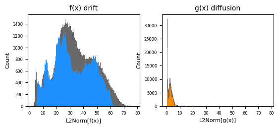
[150]:
fig, axes = cp.plot(
    nplots=2,
    ncols=2,
    height=0.5,
    width=0.5,
    wspace=0.2,
    title=["f(x) drift", "g(x) diffusion"],
    x_label=["L2Norm[f(x)]", "L2Norm[g(x)]"],
    y_label=["Count", "Count"],
)
b2 = axes[0].hist(model.adata.obs["drift"], bins=210, color="dimgrey")
b1 = axes[0].hist(model.adata.obs["smooth.drift"], bins=210, color="dodgerblue")

b2 = axes[1].hist(model.adata.obs["diffusion"], bins=210, color="dimgrey")
b1 = axes[1].hist(model.adata.obs["smooth.diffusion"], bins=210, color="darkorange")
Compute velocity graph and plot#
We’ll use the velocity components we’ve just computed to compute the velocity graph that will ultimately enable us to build a low-dimension vector field.
Note: Since we’ve performed these operations on the model.adata object, we’ll use that in this function, directly.
The following is the plot shown in Figure 2b of the manuscript.
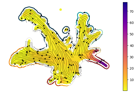
Velocity stream plots#
First, plot with un-smoothed diffusion.
[23]:
fig, axes = cp.plot(1, 1, height=1, width=1.2, del_xy_ticks=[True], delete="all")
ax = axes[0]
axes = cp.umap_manifold(
    adata,
    groupby="Cell type annotation",
    c_background=larry_cmap,
    ax=ax,
    s_background=350,
    s_cover=200,
)
sdq.pl.velocity_stream(
    model.adata,
    c="diffusion",
    cutoff_percentile=0.1,
    ax=ax,
    scatter_zorder=101,
    stream_zorder=201,
    scatter_kwargs={"rasterized": True},
)
plt.savefig("LARRY.example_velocity_stream.svg", dpi=500)
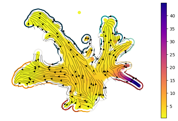
Next, plot with the smoothed diffusion:
[24]:
fig, axes = cp.plot(1, 1, height=1, width=1.2, del_xy_ticks=[True], delete="all")
ax = axes[0]
axes = cp.umap_manifold(
    adata,
    groupby="Cell type annotation",
    c_background=larry_cmap,
    ax=ax,
    s_background=350,
    s_cover=200,
)
sdq.pl.velocity_stream(
    model.adata,
    c="smooth.diffusion",
    cutoff_percentile=0.1,
    ax=ax,
    scatter_zorder=101,
    stream_zorder=201,
    scatter_kwargs={"rasterized": True},
)
plt.savefig("LARRY.example_velocity_stream.smooth.svg", dpi=500)
Compute a composite velocity from decomposed drift and diffusion#
[99]:
fx = model.adata.obs["smooth.drift"]  #  * 0.1
gx = model.adata.obs["smooth.diffusion"]
vx = fx * 0.1 + gx

velo_df = pd.DataFrame({"fx": fx, "gx": gx, "vx": vx})
vmax = velo_df.max()

f_cmap = cp.tl.custom_cmap(max_color=cp.tl.convert_matplotlib_colorname("dodgerblue"))
g_cmap = cp.tl.custom_cmap(max_color=cp.tl.convert_matplotlib_colorname("darkorange"))
v_cmap = cp.tl.custom_cmap(max_color="#7678ed")
UMAP plots: Supplementary Figure 4a#
[131]:
fig, axes = cp.plot(3, 3, height=2, width=2.4, del_xy_ticks=[True], delete="all")
xu = model.adata.obsm["X_umap"]
cmaps = [f_cmap, g_cmap, v_cmap]

for ax in axes:
    _ax = cp.umap_manifold(
        model.adata,
        groupby="Cell type annotation",
        c_background=larry_cmap,
        ax=ax,
        s_background=350,
        s_cover=200,
    )

for en, col in enumerate(velo_df):
    ax = axes[en]
    c = velo_df[col].values
    c_idx = np.argsort(c)
    img = ax.scatter(
        xu[c_idx, 0],
        xu[c_idx, 1],
        c=c[c_idx],
        zorder=300,
        vmin=0,
        rasterized=True,
        cmap=cmaps[en],
    )
    plt.colorbar(img)
plt.savefig("decomposed_velocity.svg", dpi=250)
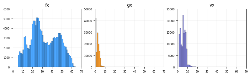
Histograms: Supplementary Figure 4b#
[138]:
colors = ["dodgerblue", "darkorange", "#7678ed"]
fig, axes = cp.plot(
    3, 3, wspace=0.2, height=0.5, width=0.5, title=velo_df.columns.tolist()
)
xlims = [70, 50, 60]
ylims = [6000, 50_000, 25_000]
for en, col in enumerate(velo_df.columns):
    ax = axes[en]
    ax.hist(
        velo_df[col],
        bins=(50),
        color="w",
        alpha=1,
        ec="None",
        zorder=4,
    )
    ax.hist(
        velo_df[col], bins=(50), color=colors[en], alpha=0.8, ec="k", zorder=5, lw=0.25
    )
    ax.set_xlim(0, 70)  # , xlims[en])
    ax.set_ylim(0, ylims[en])
    ax.grid(True, c="lightgrey", lw=0.25, zorder=0)
    [spine.set_lw(0.5) for spine in ax.spines.values()]
    ax.xaxis.set_tick_params(width=0.5)
    ax.yaxis.set_tick_params(width=0.5)
plt.savefig("histogram.velo_decomposed.svg", dpi=500)