Figure 4G

Import packages

import anndata
import ezplot
import matplotlib.pyplot as plt
import pandas as pd
import glob
import pathlib
import seaborn as sns
import sklearn.cluster
import numpy as np
import matplotlib.cm as cm

Define helper functions

def read_gene_velocity_corr(idx: int, version: int):
    base_path = f"./version_{version}_gene_velocity_corr/{idx}.*.csv"
    paths = glob.glob(base_path)

    DataFrames = {}
    for path in paths:
        fpath = pathlib.Path(path)
        fate = fpath.name.split(".")[1]
        if fate != "Undifferentiated":
            DataFrames[fate] = pd.read_csv(path, index_col = 0)

    return DataFrames

def _adjust_colnames(data, fate: str = "Monocyte"):
    df = data[fate].copy()
    df.columns = [f"{fate}.{key}" for key in df.columns]
    return df

Two fates

For the two-fate example, we’ll use idx=19977 (v3)

data = read_gene_velocity_corr(idx = 19977, version = 3)
df = pd.concat([_adjust_colnames(data, "Monocyte"), _adjust_colnames(data, "Neutrophil")], axis = 1)
df

	Monocyte.f.corr	Monocyte.f.pval	Monocyte.g.corr	Monocyte.g.pval	Neutrophil.f.corr	Neutrophil.f.pval	Neutrophil.g.corr	Neutrophil.g.pval
gene_ids
1110002J07Rik	0.246731	0.119912	0.594733	4.121254e-05	0.025470	8.744020e-01	0.406625	8.333975e-03
1110032F04Rik	0.537274	0.000292	0.322823	3.952964e-02	0.533234	3.310762e-04	0.298061	5.838780e-02
1500002F19Rik	0.199835	0.210322	-0.192597	2.276558e-01	-0.679190	1.050207e-06	-0.932045	8.675594e-19
1500026H17Rik	-0.144147	0.368571	-0.669251	1.718679e-06	-0.656420	3.160551e-06	-0.927592	2.872365e-18
1600010M07Rik	-0.666030	0.000002	-0.851748	1.666314e-12	-0.297194	5.915940e-02	-0.664837	2.126375e-06
...	...	...	...	...	...	...	...	...
Zmpste24	0.667209	0.000002	0.913492	8.110006e-17	-0.876496	5.967734e-14	-0.819266	5.826618e-11
Zmynd15	-0.038569	0.810783	0.464953	2.192460e-03	0.329221	3.556725e-02	0.801130	3.157972e-10
Znfx1	-0.624361	0.000013	-0.976683	1.131776e-27	-0.771510	3.547780e-09	-0.961632	1.633703e-23
Zscan2	0.462753	0.002316	0.499486	8.850821e-04	0.349633	2.504204e-02	0.112174	4.850126e-01
Zyx	-0.538328	0.000283	-0.969048	2.649156e-25	-0.642644	5.891798e-06	-0.944852	1.659873e-20

2492 rows × 8 columns

Read table of transcription factors (from Weinreb2020)

def get_tf_table(df):
    tf_df = pd.read_table(
        "/Users/michaelvinyard/tf_list.txt",
        usecols=[1, 2, 3],
        index_col = 0,
        header=None,
        names=['idx', 'gene_name', 'description'],
    )
    return df.loc[df.index.isin(tf_df['gene_name'].tolist())]

tf_df = get_tf_table(df)
tf_df = tf_df.filter(regex = "corr").copy()

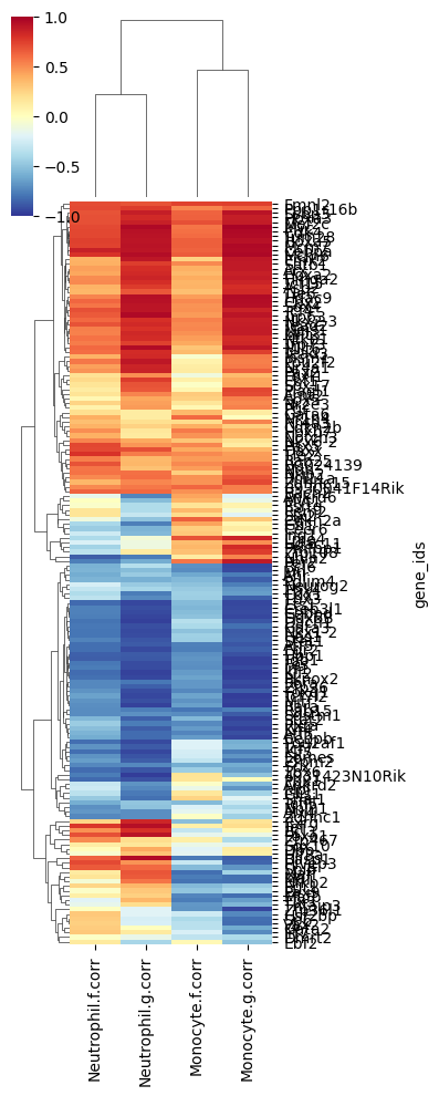
Plot heatmap for Figure 4G

cg = sns.clustermap(
    tf_df,
    vmin = -1,
    vmax = 1,
    cmap = cm.RdYlBu_r,
    figsize = (4, 10),
    rasterized = True,
    yticklabels = tf_df.index,
)
plt.savefig("Figure4G.svg")

tf_df.to_csv("scdiffeq.SupplementaryTable6.csv")